Guide to surface x-ray diffraction analysis
Here are some walkthroughs to aid in the analysis of surface x-ray diffraction measurements
Crystal Truncation Rods |
Reflectivity |
In-plane omega scans |
|
|
|
Specular 00L rods |
GIWAXS |
GISAXS |

|
|
|
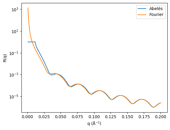
Reflectivity ( low angle \(\theta-2\theta scans\))
- These are specular measurements taken at low \(\theta\) values near the critical edge of your sample, and can be analysed with the following steps:
Reduce the data to a 1D reflecitivty profile, which can be done using the islatu package
use a program such as GenX to model the reflectiity profile
Specular 00L rod ( \(\theta-2\theta scans\))
- These are specular measurements taken at higher \(\theta\) values, away from the critical edge of your sample. These can be analysed using the following steps:
Reduce the data to a 1D profile, which can be done using the islatu package
Peak positions and widths can be used for quantitative analysis of your 00L profile
Out-of-plane strain can be calculated by analysing HKL positions
The 00L profile can be loaded into fitting programs such as ROD for full structure fitting. There are also options for automating ROD
Note
For a full structural fit, the specular 00L profile is usually combined with off-specular crystal truncation rod measurements.
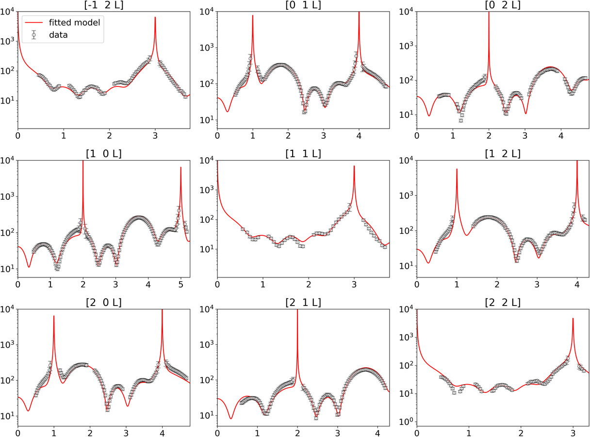
Crystal truncation rod data
- These are measurements taken with a fixed incident angel, and along the L direction at a variety of HK positions, which can take both integer and fraction positiosn of H and K. These can be analysed using the following steps:
Map the data from raw images into HKL space, which can be done using the fast_rsm package
Reduce the 3D HKL volumes data into 1D profiles, which can be done using the binoviewer package (under development)
The off-specular CTR profiles can be loaded into fitting programs such as ROD for full structure fitting. There are also options for automating ROD
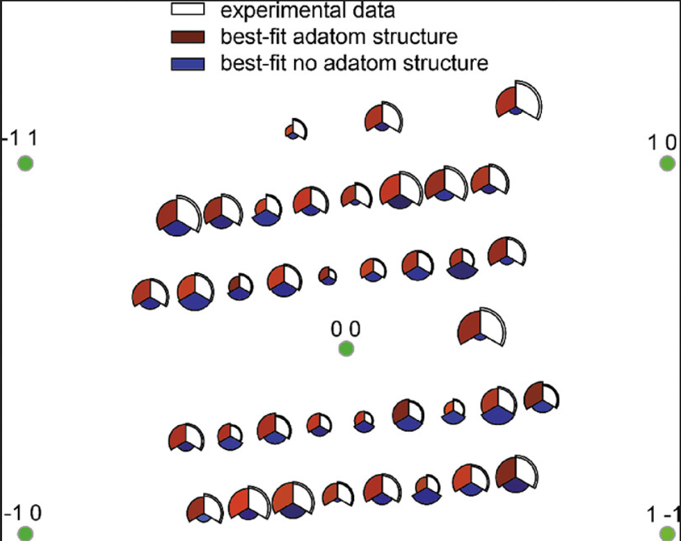
In-plane omega scans
- These are measurements taken at fixed very low L value, and are collected by rocking the sample around it azimuthal axis. These can be analysed using the following steps:
Reduce the raw data to individual intensities for each HK position. See extra information on reducing omega scan data
The 00L profile can be loaded into fitting programs such as ROD for full structure fitting - Note: these are usually combined with off-specular crystal truncation rod measurements. There are also options for automating ROD
Note
For a full structural fit, the in-plane omega scans are usually combined with off-specular crystal truncation rod measurements
Grazing incidence wide angle x-ray scattering
- These are measurements taken with a large detector position close to the sample, and usually require some form of azimuthal integration. These can be processed in the following steps:
obtain calibration information so you know the detector distance from your sample
azimuthally integrated the data or map the data into 2D co-ordinate system (Q_parallel Vs Q_Perpendicular, exit angles)
both of these steps can be done using the pyFAI python package. For Diamond data sets the fast_rsm package already makes use of the pyFAI module.
Grazing incidence small angle x-ray scattering
Links to website resources
ANArod project from ESRF - https://www.esrf.fr/computing/scientific/joint_projects/ANA-ROD/